SYSTEM COMPONENTS

PINNED ROD
Element COMPONENTS

General

The Matrix Structural Analysis solution is also called Finite Element Analysis, or the Displacement Method, or the Stiffness Method (as opposed to the Flexibility Method.)

The system consists of nodes (specific locations in a Cartesian coordinate system), and elements (structural members) that connect the nodes. All nodes in a structural system must be connected to a least one element, and all elements must be connected to a least two nodes.

The coordinate system defining the nodes is called the Global Coordinate System. It is the common coordinate system to which all the element local coordinate systems must be resolved in order to effect a solution.

Each element has its own Local Coordinate System. Internal forces and deformations (deflections and rotations) in their local coordinate system are related to the global coordinate system by means of the Transformation Matrix.

External loads are applied to nodes only.

Defining the Global Coordinate System.

Coordinate systems define points in space. The space can be two-dimensional or three-dimensional. The coordinate system can rectangular (x, y, z), spherical (a, b, g, r), or cylindrical (a, b, r). In this discussion we will display the rectangular (x, y, z) system.

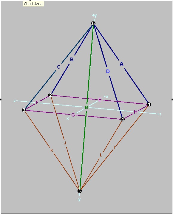
In the rectangular X, Y, Z coordinate system to the right, there are six nodes, numbered 1 through 6.

There are thirteen elements connected to the six nodes, labeled A through M

Define the Nodes of the structural system in the Global Coordinate System.

The Nodes are very simple to define, In the table to the right, all there is to do is give each node a unique label, and list its coordinates. In this example we use the numbers 1 through 6 to label each of the six nodes. Then we list the X, Y, Z (global) coordinates for each node.

We will differentiate the global coordinate system from a local coordinate system by using upper case for the global system, and lower case for a local system.

node	X	Y	Z
1	20	0	20
2	20	0	-20
3	-20	0	-20
4	-20	0	20
5	0	20	0
6	0	-20	0

Defining the structural elements
Defining an element's location and connectivity is also very simple -- just give the element a label, and define which nodes it connects to.

In the example to the right (and depicted above), the elements are all pinned bars, with two nodes -- a beginning (i) node and an ending (j) node.

From this information, and the coordinates of each node, we can calculate the transformation matrix that resolves the element forces and displacements from their local coordinate system into the global coordinate system. This is necessary so that we can sum all the forces acting on a node in a common (global) coordinate system. And we also equate nodal displacements to element displacements in a common (global) coordinate system.

*element*	i	j
A	1	5
B	2	5
C	3	5
D	4	5
E	1	2
F	2	3
G	3	4
H	4	1
I	1	6
J	2	6
K	3	6
L	4	6
M	5	6

We also need each element's physical properties, such as Modulus of Elasticity (E), Cross-sectional Area (A), and Length (L). For the example displayed (pinned rods) that's all we need. But if the elements were beams, we would need more information, such as Moments of Inertia (Iy, Iz, Jx).

For the example (pinned rods), we input E and A for each element, but we calculate L from the ith and jth coordinates as follows:

1) L = [(X_j - X_i)² + (Y_j - Y_i)²+ (Z_j - Z_i)²]^1/2Remember that Matrix Structural Analysis is a numerical solution, and every physical property requires a numerical value. And, while it is common for all the elements to be the same material, they can all be different,. which is why we identify each with a subscript related to the individual element.

Also important is that we are dealing with small displacement and linear theory, and that buckling of slender rods under compression is not accounted for.

Rods

element i j E A L

A 1 5 E_A A_A L_A

B 2 5 E_B A_B L_B

C 3 5 E_C A_C L_C

D 4 5 E_D A_D L_D

E 1 2 E_E A_E L_E

F 2 3 E_F A_F L_F

G 3 4 E_G A_G L_G

H 4 1 E_H A_H L_H

I 1 6 E_I A_I L_I

J 2 6 E_J A_J L_J

K 3 6 E_K A_K L_K

L 4 6 E_L A_L L_L

M 5 6 E_M A_M L_M

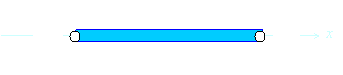
A Pinned Rod in its local coordinate system.

A pinned rod is the simplest element that exists. We are going to us it to illustrate the general theory of the stiffness and transformation matrices of an element. It is simply easier to explain by using an example.

On the depiction to the right is a pinned rod, lying along its local x axis, with the ith node at (or near) the origin, and the jth node at a point further away along the positive x-axis.

A local force f_i is applied to the ith end of the rod, and a counter force f_j is applied to the jth end of the rod.

Please note that a pinned rod can only sustain forces along its axis.

The Stiffness Matrix of a Pinned Rod

The material properties of the rod are E, A, and L, where L = x_j - x_i

If we sum forces in the x direction, we get

SF_x = 0 = f_i + f_j = 0
or
f_i = -f_j

The displacement u_j at the jth end of the rod, is equal to the displacement u_i plus the deformation d of the rod due to the forces applied, which is
d = f_j L/(EA)

The equation then becomes u_j = u_i + d
or
2) u_j = u_i + f_j L/(EA)

Likewise, we can determine the displacement of u_i given u_j, which is
3)   u_i = u_j + f_i L/(EA)

If we solve Equations 2) and 3) for f_i and f_j, we get the following:

f_i = EA/L [u_i - u_j]
                                                                      or in matrix form      4)
f_j = EA/L [-u_i + u_j]

or in abbreviated matrix notation f = k u                        where     5)

k is the element's stiffness matrix.

Later we will derive this more rigorously and by different methods, but for now we want to move on and derive the transformation matrix, then use this in an example solution.

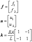
The Transformation Matrix of a Pinned Rod

In order to perform structural analysis, we have to transform all forces and deflections so they align with a common (global) coordinate system.

To the right is a figure that depicts how the transformation matrix is derived from the nodes that the element is connected to.

Remember that we already input the X, Y, and Z coordinates for both the ith and jth nodes for any element.

And remember that we calculated L from Equation 1), above.

The first step is to calculate the direction cosines.

Direction Cosines (l)
Direction cosines are coefficients that allow us to render any vector in space into its orthogonal (x, y, z) components. The vectors in our structural system are the force vectors and the displacement vectors.

For our matrix structural analysis example, the direction cosines are very simple to calculate from the global coordinates assigned to our element, as to the right:

These direction cosines (which are dimensionless may be applied directly to any vector in our system, and in particular to the force vectors, and displacement vectors of this element.

l_X = (X_j - X_i) / L
6) l_Y = (Y_j - Y_i) / L
l_Z = (Z_j - Z_i) / L

l_X is the cosine of the angle formed by the rod and the X axis.

l_Y is the cosine of the angle formed by the rod and the Y axis.

l_Z is the cosine of the angle formed by the rod and the Z axis.

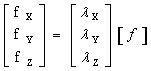
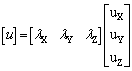
For the force vector f, and the displacement vector u, in our local x coordinate system (it is a one-dimensional element), we transform it to our global X, Y, Z system as presented to the right:

If we define l as [l_X l_Y l_Z] or

then we can define l^T as [l_X l_Y l_Z]^T or

l= [l_X l_Y l_Z]

We apply the above transforms to the forces and deflections at each node independently as follows:

f_i = l^Tf_i   and u_i = lu_i
and                                     or, in combined in one matrix statement
f_j = l^Tf_j   and u_j = lu_j

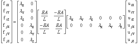
The above in fully expanded form

Degrees of Freedom
Note that we are still referring to a single rod element. What we have done is transform the single degree of freedom (at each element node) in the local coordinate system to a three degrees of freedom (at each element node) in the global coordinate system.

Note also that while generally a global node can have six degrees of freedom (three translations - in the X, Y, and Z directions, and three rotations - about the X, Y, and Z axes), pinned-rods cannot take rotations (associated with applied moments.) So a global node with only pinned rods attached to it will only have three degrees of freedom - translations in the X, Y and Z directions.

The Globalized Pinned Rod Element
We need to have a globalized pinned element so that we can connect rods together in a structural system and enforce equations of equilibrium (on forces) at the nodes, and equations of compatibility (on deflections) at the nodes. We will address the equations of equilibrium and compatibility in the next chapter. next -- but before we do, we consolidate the above element equations into its globalized form, below.

f = l^T k l u

Note that the pinned rod started out as a 2 by 2 matrix (a single degree of freedom at each end) in its local coordinate system, and ended up as a 6 by 6 matrix (three degrees of freedom at each end) in the global coordinate system.

The next step is to create the equilibrium and compatibility matrices, and those are only meaningful for a structural system.
This is illustrated in the next chapter on a
Structural System of Pinned Rods